
Aerial LiDAR measures distances. That is a difference in kind from imagery, which records light intensity, and it explains most of what follows.
Where a satellite image shows what a surface looks like, a LiDAR survey states where it sits in space. This article sets out the principle, the derived products, the applications and the annotation work this modality requires. It opens a series devoted to it.
The measurement principle of aerial LiDAR
An onboard sensor emits laser pulses towards the ground. It measures the return time of each echo, which gives a distance. Three distinct elements combine to convert that distance into an absolute position. The aircraft’s position, supplied by a high precision satellite receiver. Its orientation, supplied by an inertial unit. And the pulse emission angle, known from the sensor’s mechanics. The result is a point cloud, each point carrying three coordinates and several attributes. It is not an image but a set of point measurements, which changes every tool and every method. One important consequence follows. A survey’s quality depends as much on the positioning system as on the laser sensor itself, and a trajectory error produces a distortion nothing later corrects.What a point contains
These attributes condition the annotation work. Each point carries more than its position alone. The three-dimensional coordinates are the primary information. Intensity measures the energy of the returned echo, information related to the nature of the surface and to the measurement geometry, usable with caution. The echo number and total echo count indicate whether the pulse met several successive surfaces, decisive information in vegetated areas the next section details. The scan angle indicates the emission direction, useful for understanding certain distortions. The flight line number permits distinguishing passes, information needed for consistency checking between strips. And the classification, where it exists, assigns each point to a category, ground, vegetation or building notably, which is precisely the object of annotation.Multiple returns
This property distinguishes aerial LiDAR from every other modality. It explains an important part of its value. A laser pulse meeting a vegetation canopy divides. Part reflects off the upper leaves, another passes through and reflects lower, part sometimes reaches the ground. The sensor records several echoes for a single pulse, producing information about vertical structure that neither imagery nor radar supplies. Three important consequences follow. The ground is measurable under forest cover, a property founding the forestry use of this technology. The vertical structure of vegetation is described, permitting height, density and stratification to be estimated. And the penetration rate varies strongly with canopy density and season, a survey under leaf reaching the ground markedly less than one taken leaf-off. That last observation has practical reach. The acquisition season determines what a survey permits, and a project concerning ground under forest must acquire leaf-off.The derived products of aerial LiDAR
A raw point cloud is rarely the expected deliverable. Three products derive from it, which an article in this series details. The digital terrain model describes bare ground elevation, obtained by retaining only points classified as ground and interpolating between them. The digital surface model describes the elevation of the top of whatever covers the ground, vegetation and buildings included. And the canopy or normalised height model describes the difference between the two, meaning the height of objects above the ground. One important observation runs across those three products. They depend entirely on the classification of the points, which makes the classification stage the determinant of their quality rather than the reverse.Classification, the heart of the work
It consists of assigning a class to each point. An article in this series details its difficulties. A standard nomenclature exists in the field’s exchange format and it comprises base classes, ground, low, medium and high vegetation, building, water, bridge and noise notably. Three difficulties dominate this classification work. Volume, a survey covering a few square kilometres containing tens of millions of points, which precludes manual point-by-point handling. Ambiguity at interfaces, a point sitting at the limit between ground and low vegetation or between vegetation and building belonging to a convention rather than to an obvious fact. And three-dimensionality, an annotator having to navigate a space rather than examine an image, which requires different tooling and different practice. One practical consequence follows. LiDAR annotation proceeds by selecting groups of points rather than designating individual ones, and quality depends on the relevance of those selections more than on pointwise precision.What distinguishes aerial LiDAR from imagery
Six differences structure the comparison and an article in this series details it. The measurement is direct in elevation, where imagery must infer it through stereoscopy or cast shadow. Penetration of vegetation cover is possible, a property no passive imagery holds. Independence from illumination is total, the sensor emitting its own signal, which permits night acquisition. Colour information is absent, a LiDAR point carrying no colour, which limits identification of surface nature. Coverage is more expensive, an airborne acquisition not covering the areas a satellite covers. And the data is bulkier per unit area, which weighs on storage and processing. One observation runs across those six differences. The two modalities are complementary rather than competing, one measuring geometry and the other describing appearance, which an article in this series develops.Point density
This parameter governs what an aerial LiDAR survey permits. An article in this series is devoted to it. Density is expressed in points per square metre and it follows from the emission frequency, the flight altitude and the aircraft’s speed. Three density bands serve distinct uses. Low density suits a terrain model over wide areas. Medium density suits forestry and building mapping. And high density suits detailed infrastructure modelling. An economic trade-off accompanies that choice. Density conditions acquisition cost, flight speed and therefore area covered per hour, which makes it a project’s first decision. One consequence for annotation deserves flagging. Classification cost grows with density, a dense survey containing more points to handle for the same area, which makes density decisive on both sides.Acquisition platforms
Three carriers coexist and their choice determines area covered as much as precision obtained. The aircraft covers wide areas at altitudes from several hundred to a few thousand metres, with moderate density and a low cost per unit area. It is the platform of national coverage programmes. The helicopter flies lower and slower, producing higher density over restricted footprints, a configuration suited to linear infrastructure monitoring. And the drone descends further, producing very high densities over limited areas, with modest deployment cost and regulatory flight constraints. A fourth platform deserves flagging although it sits outside the aerial frame. Satellite LiDAR exists and it works by sampling along tracks rather than by continuous coverage, which makes it an instrument of global measurement rather than a mapping tool. One practical consequence follows for an aerial LiDAR project. The platform choice precedes the density choice, the two being linked, and it determines whether regional coverage or a local survey is feasible.The main applications of aerial LiDAR
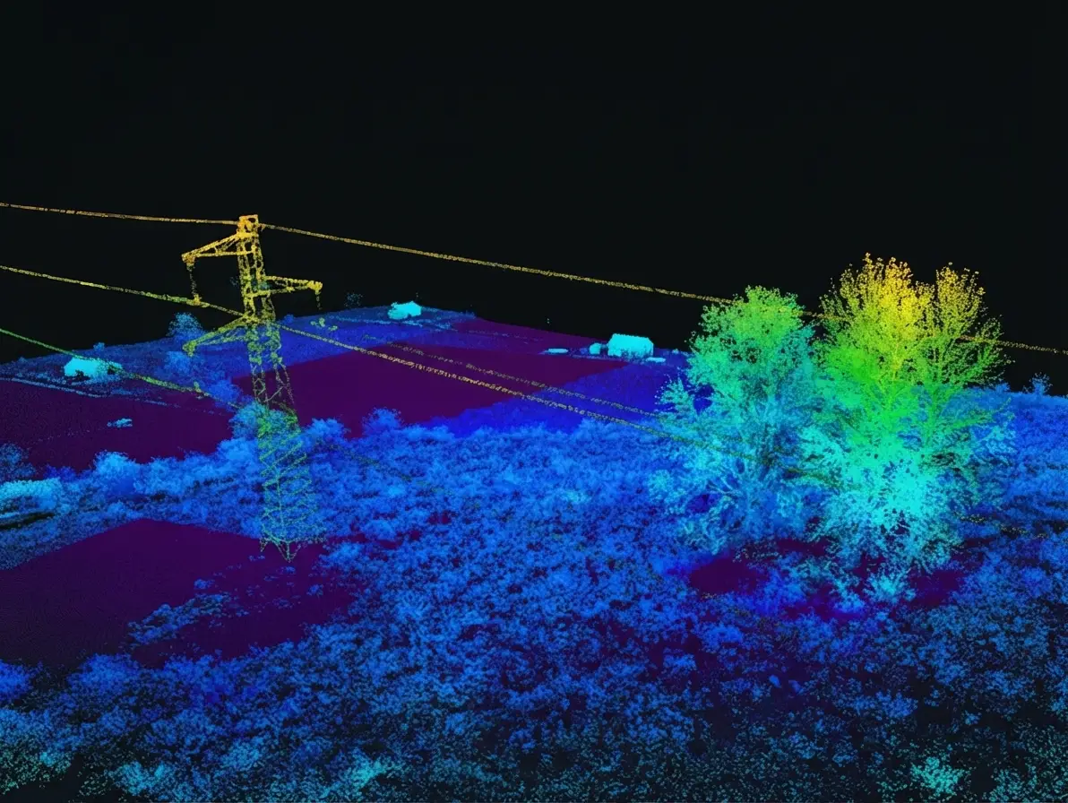
Five domains employ it. Several are the subject of dedicated articles in this series. Forestry exploits canopy penetration to measure heights, estimate volumes and characterise structure. Power network management exploits the geometric precision to measure distances between vegetation and conductors. Urban planning exploits the three-dimensional description of buildings to feed territorial models. Hydrology exploits the terrain model to model flows and flood-prone areas. And archaeology exploits the same capability to reveal structures masked by vegetation, a spectacular and economically marginal use.National programmes
This development changes access to aerial LiDAR data. An article in this series details it. Several countries have launched national LiDAR coverage programmes, producing surveys at homogeneous density across a whole territory and distributing them under open licence. Three consequences follow. Acquisition cost disappears for projects within covered areas, which shifts the economics towards processing. An automatic classification generally accompanies this data, of variable quality and often insufficient for a precise use. And a homogeneous reference becomes available, which eases comparisons and time series. One important observation accompanies that. The classification delivered with these programmes is a starting point rather than a finished product, and most of the work consists of correcting and refining it rather than producing it.Formats and tooling
One exchange format dominates this field. Knowing it is a prerequisite. The standard format stores points with their attributes and a compressed variant considerably reduces volume without loss, which makes it the default choice for archiving and exchange. Three families of tool intervene in this field. Point cloud viewers and editors, for exploration and annotation. Processing libraries, for filtering, automatic classification and derived product generation. And geographic information systems, for integrating results with other data. One difficulty deserves flagging. Three-dimensional annotation tooling is markedly less mature than its two-dimensional equivalent, which an article in this series develops and which constitutes a barrier to entry as much as a difficulty.The processing chain
Six stages separate a raw survey from a usable product and omitting them produces distinct difficulties. Trajectory computation combines positioning and inertial data to reconstruct the aircraft’s exact path, an operation whose quality conditions everything else. Direct georeferencing converts distance measurements into absolute coordinates, applying the trajectory and the scan angles. Strip adjustment corrects discrepancies between adjacent flight lines, two passes over one area never coinciding exactly. Noise filtering discards spurious echoes, birds, atmospheric particles and multiple reflections. Classification assigns a class to each point, a stage this series develops. And derived product generation interpolates surfaces from the classified points. One important observation runs across those six stages. The first three belong to the acquisition supplier and the last three to processing, a division determining where responsibility sits in case of defect and worth clarifying contractually.What aerial LiDAR annotation requires
Four requirements distinguish this work. They justify a competence of its own. Three-dimensional navigation, an annotator having to move through a space, change viewpoint and cut sections to understand a configuration. Reading structure, recognition proceeding through geometric form and relative arrangement rather than through appearance. Managing volume, a selection covering thousands of points and precision depending on the relevance of the selection criterion. And ground knowledge, distinguishing a bank from a low wall or a bush from a vehicle requiring a familiarity geometry alone does not supply. Those four requirements explain why LiDAR annotation competence does not follow from image annotation competence, a distinction the preceding series documented for other modalities.The cost of an aerial LiDAR project
A breakdown deserves setting out because the distribution of lines differs markedly from an imagery project. Five lines compose it and an article in this series details them. Acquisition, nil where a national programme covers the area and substantial otherwise, an airborne campaign carrying a significant fixed cost. Storage and processing, heavier than in imagery through volume, a dense survey over a few square kilometres exceeding tens of gigabytes. Classification, the dominant line where acquisition is free, and whose cost grows with density and class count. Quality control, which the corresponding article shows requires methods specific to three-dimensionality. And derived product generation, a modest and largely automatable line once the classification is established. One important observation follows. Where an imagery project sees its cost dominated by annotation whatever the source, an aerial LiDAR project shifts from an acquisition-dominated profile to a classification-dominated one according to whether the area is covered by a public programme.What aerial LiDAR does not supply
An honest reading requires setting out the limits, failing which a project is badly sized. Surface nature largely escapes this modality. A point carries no colour and intensity informs imperfectly, which makes distinguishing two materials of similar geometry difficult. Temporal coverage is low. An airborne acquisition is scheduled and costs, which precludes the dense series a satellite produces, and most territories hold only one or two surveys. Water surfaces are poorly measured. The laser used in topographic aerial LiDAR is absorbed by water, producing zones with no return, and bathymetry requires a different sensor. And vertical surfaces are undersampled. A sensor looking downwards reaches facades poorly, which limits detailed urban modelling and explains the recourse to oblique or terrestrial acquisitions. Those four limits lead to a recommendation. Establishing at scoping whether the information sought is geometric or descriptive determines whether this modality suits, a question taking a minute and eliminating badly directed projects.Questions to ask at scoping
Five questions scope an aerial LiDAR project and they are asked in one meeting. Is the information sought geometric. A negative answer points to imagery and avoids a badly launched project. Does a survey exist over the area. Its availability radically changes the project’s economics and the type of work required. What existing classification accompanies that survey. Assessing it on a sample determines whether the work is correcting or producing. Is ground under canopy needed. That requirement imposes a leaf-off acquisition and rules out summer surveys. And what density does the use require. That answer determines the platform, the acquisition cost and the classification cost simultaneously. Those five answers determine feasibility, source, type of engagement and budget. Asking them before drafting a proposal produces a document describing the right work.Where to start
Five steps structure a project’s start and their order matters. Frame the operational question as a decision, which determines the classes needed and the density required. Check for an existing survey over the area, a national programme potentially removing the acquisition cost. Assess the existing classification on a sample, which determines whether the work is correcting or producing. Fix the nomenclature and the interface conventions before any annotation. And run a pilot over a small area to establish a throughput and reveal ambiguous cases.What this modality offers a data provider
Three commercial consequences emerge from this survey. The first is that classification is this field’s bottleneck. Derived products depend on it entirely, delivered automatic classifications are insufficient, and correction represents most of the remaining work, which places a provider at the point where value is created. The second is that three-dimensional competence is scarce. It does not follow from image annotation, it requires its own training, and few actors hold it, a configuration the preceding series identified as the most favourable. And the third is that national programmes create demand rather than removing it. Free coverage classified roughly makes projects accessible that were not, and each requires a refinement the programme does not supply. That third consequence deserves emphasis. Contrary to intuition, the free distribution of aerial LiDAR data widens the processing market instead of reducing it, exactly as free satellite imagery did for image annotation.Reading a survey’s specification
One practical skill deserves setting out, since a project generally begins by receiving a survey rather than commissioning one. Six items in a specification determine what the data permits, and each is stated in the accompanying metadata. The nominal point density, which bounds what objects are resolvable and which is an average rather than a guarantee at every location. The acquisition date and season, which determines canopy penetration and therefore ground coverage under forest. The vertical and horizontal accuracy, generally stated separately, the vertical being the better of the two in aerial LiDAR. The classification scheme applied, and critically whether it was manually verified or purely automatic. The strip overlap and whether adjustment was performed, which indicates whether discrepancies between flight lines were corrected. And the coordinate reference system and vertical datum, whose mismatch with a project’s other data is a frequent and silent source of error. One observation completes those six. A specification stating a density and an accuracy while saying nothing about the classification method is describing the acquisition rather than the product, and the difference matters entirely for a project intending to use the classes.Common mistakes
These failures recur often enough that naming them is usually enough to avoid them.- Confusing terrain model with surface model.
- Acquiring leaf-on for a project concerning ground under forest.
- Choosing a density without considering its effect on annotation cost.
- Treating the classification delivered with a national programme as a finished product.
- Using image annotators without three-dimensional training.
- Neglecting the conventions at interfaces between classes.
- Exploiting intensity without accounting for measurement geometry.
- Ignoring discrepancies between flight strips.
- Generating a terrain model without verifying the ground classification.
- Expecting from LiDAR surface nature information it does not carry.